数据挖掘 | 决策树/随机森林应用于鸢尾花分类

本文最后更新于：2021年5月8日凌晨

# 数据挖掘 | 决策树/随机森林应用于鸢尾花分类

本文主要分为四个部分：

数据集探索（了解数据内容）
各维度数据可视化（绘制各维度直方图和散点图矩阵，但不限于此）
决策树模型、可视化及调参（训练决策树模型，可视化决策树，尝试不同决策树参数对分类准确度的影响）
扩展实验（随机森林模型）

01 / 数据集和模型简介

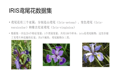
鸢尾花数据集

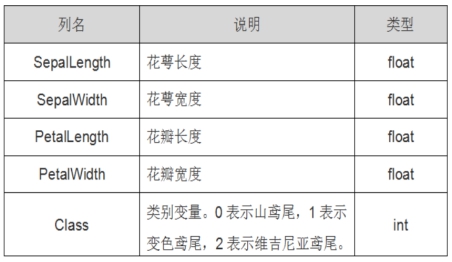
鸢尾花数据集内包含 3 类（iris-setosa, iris-versicolour, iris-virginica）共 150 条记录，每类各 50 个数据，每条记录都有 4 项特征：花萼（Sepal）长度、花萼宽度、花瓣（Petal）长度、花瓣宽度。可以通过这4个特征对鸢尾花进行聚类或者预测鸢尾花卉属于中的哪一品种。

决策树模型

决策树（decision tree）是一种描述对实例进行分类的树形结构。

决策树由结点和有向边组成。结点有两种类型：内部结点和叶结点。内部结点表示一个特征或属性，每个分支代表这个特征属性在某个值域上的输出，叶结点表示一个类。

使用决策树进行决策的过程就是从根结点开始，测试待分类项中相应的特征属性，并按照其值选择输出分支，直到到达叶结点，将叶结点存放的类别作为决策结果。

02 / 探索性数据分析

数据集探索

导入工具包和鸢尾花数据集

import matplotlib.pyplot as plt
import pandas as pd
import numpy as np
from sklearn.datasets import load_iris

from sklearn import tree
from sklearn import metrics
from sklearn.tree import DecisionTreeClassifier
from sklearn.ensemble import RandomForestClassifier
from sklearn.model_selection import train_test_split

加载鸢尾花数据集

from sklearn.datasets import load_iris
iris_dataset = load_iris()

查看数据集对象的属性和方法

dir(iris_dataset)

[‘DESCR’,
‘data’,
‘feature_names’,
‘filename’,
‘frame’,
‘target’,
‘target_names’]

查看数据集标签名

iris_dataset.target_names

array([‘setosa’, ‘versicolor’, ‘virginica’], dtype=’<U10’)

查看数据集标签

iris_dataset.target

array([0, 0, 0, 0, 0, 0, 0, 0, 0, 0, 0, 0, 0, 0, 0, 0, 0, 0, 0, 0, 0, 0,
0, 0, 0, 0, 0, 0, 0, 0, 0, 0, 0, 0, 0, 0, 0, 0, 0, 0, 0, 0, 0, 0,
0, 0, 0, 0, 0, 0, 1, 1, 1, 1, 1, 1, 1, 1, 1, 1, 1, 1, 1, 1, 1, 1,
1, 1, 1, 1, 1, 1, 1, 1, 1, 1, 1, 1, 1, 1, 1, 1, 1, 1, 1, 1, 1, 1,
1, 1, 1, 1, 1, 1, 1, 1, 1, 1, 1, 1, 2, 2, 2, 2, 2, 2, 2, 2, 2, 2,
2, 2, 2, 2, 2, 2, 2, 2, 2, 2, 2, 2, 2, 2, 2, 2, 2, 2, 2, 2, 2, 2,
2, 2, 2, 2, 2, 2, 2, 2, 2, 2, 2, 2, 2, 2, 2, 2, 2, 2])

查看数据集特征名

iris_dataset.feature_names

[‘sepal length (cm)’,
‘sepal width (cm)’,
‘petal length (cm)’,
‘petal width (cm)’]

查看数据集特征数据

iris_dataset.data

array([[5.1, 3.5, 1.4, 0.2],
[4.9, 3. , 1.4, 0.2],
[4.7, 3.2, 1.3, 0.2],

…

[6.2, 3.4, 5.4, 2.3],
[5.9, 3. , 5.1, 1.8]])

查看特征数据尺寸

iris_dataset.data.shape

(150, 4)

用pandas列出鸢尾花数据集的内容和标签

import pandas as pd
iris_df = pd.DataFrame(iris_dataset.data, columns=iris_dataset.feature_names)
iris_df['label'] = iris_dataset.target

用pandas将数据整合成 DataFrame 并展示

iris_df

sepal length (cm) sepal width (cm) petal length (cm) petal width (cm) label

0 5.1 3.5 1.4 0.2 0

1 4.9 3.0 1.4 0.2 0

2 4.7 3.2 1.3 0.2 0

3 4.6 3.1 1.5 0.2 0

4 5.0 3.6 1.4 0.2 0

… … … … … …

145 6.7 3.0 5.2 2.3 2

146 6.3 2.5 5.0 1.9 2

147 6.5 3.0 5.2 2.0 2

148 6.2 3.4 5.4 2.3 2

149 5.9 3.0 5.1 1.8 2

150 rows × 5 columns

	sepal length (cm)	sepal width (cm)	petal length (cm)	petal width (cm)	label
0	5.1	3.5	1.4	0.2	0
1	4.9	3.0	1.4	0.2	0
2	4.7	3.2	1.3	0.2	0
3	4.6	3.1	1.5	0.2	0
4	5.0	3.6	1.4	0.2	0
…	…	…	…	…	…
145	6.7	3.0	5.2	2.3	2
146	6.3	2.5	5.0	1.9	2
147	6.5	3.0	5.2	2.0	2
148	6.2	3.4	5.4	2.3	2
149	5.9	3.0	5.1	1.8	2

查看数据集各特征列的摘要统计信息

iris_df.describe()

sepal length (cm) sepal width (cm) petal length (cm) petal width (cm) label

count 150.000000 150.000000 150.000000 150.000000 150.000000

mean 5.843333 3.057333 3.758000 1.199333 1.000000

std 0.828066 0.435866 1.765298 0.762238 0.819232

min 4.300000 2.000000 1.000000 0.100000 0.000000

25% 5.100000 2.800000 1.600000 0.300000 0.000000

50% 5.800000 3.000000 4.350000 1.300000 1.000000

75% 6.400000 3.300000 5.100000 1.800000 2.000000

max 7.900000 4.400000 6.900000 2.500000 2.000000

	sepal length (cm)	sepal width (cm)	petal length (cm)	petal width (cm)	label
count	150.000000	150.000000	150.000000	150.000000	150.000000
mean	5.843333	3.057333	3.758000	1.199333	1.000000
std	0.828066	0.435866	1.765298	0.762238	0.819232
min	4.300000	2.000000	1.000000	0.100000	0.000000
25%	5.100000	2.800000	1.600000	0.300000	0.000000
50%	5.800000	3.000000	4.350000	1.300000	1.000000
75%	6.400000	3.300000	5.100000	1.800000	2.000000
max	7.900000	4.400000	6.900000	2.500000	2.000000

iris_df.info()

<class ‘pandas.core.frame.DataFrame’>

RangeIndex: 150 entries, 0 to 149

Data columns (total 5 columns):

# Column Non-Null Count Dtype

— ------ -------------- -----

0 sepal length (cm) 150 non-null float64

1 sepal width (cm) 150 non-null float64

2 petal length (cm) 150 non-null float64

3 petal width (cm) 150 non-null float64

4 label 150 non-null int32

dtypes: float64(4), int32(1)

memory usage: 5.4 KB

各维度数据可视化

通过数据可视化对数据集进行进一步的探索性分析，比如绘制各维度直方图和散点图矩阵，找出数据中的关联。

导入包，初始化绘图配置

import matplotlib.pyplot as plt
import seaborn as sns
sns.set_style("whitegrid")
# 设置颜色主题
antV = ['#1890FF', '#2FC25B', '#FACC14']

绘制各维度直方图

f, axes = plt.subplots(2,2, figsize=(16, 8), sharex=True)
sns.despine(left=True)
# sns.histplot(x=iris_df['label'],  color=antV[2], ax=axes[2, 0])
sns.histplot(x=iris_df['sepal length (cm)'], color=antV[0], ax=axes[0, 0])
sns.histplot(x=iris_df['sepal width (cm)'],  color=antV[0], ax=axes[0, 1])
sns.histplot(x=iris_df['petal length (cm)'],  color=antV[1], ax=axes[1, 0])
sns.histplot(x=iris_df['petal width (cm)'],  color=antV[1], ax=axes[1, 1])
plt.savefig("features_hist.png")
plt.show()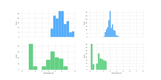

绘制各维度散点图矩阵

from matplotlib import cm
from pandas.plotting import scatter_matrix as sm
import matplotlib.pyplot as plt
import pandas as pd
cmap = cm.get_cmap('gnuplot')
s = sm(iris_df[iris_dataset.feature_names], c=antV[1],marker="o", s=40,hist_kwds={ 'bins': 15}, figsize=(12, 12), cmap=cmap, alpha=0.4)
plt.savefig("feartures_scatter_mat.png")
plt.show()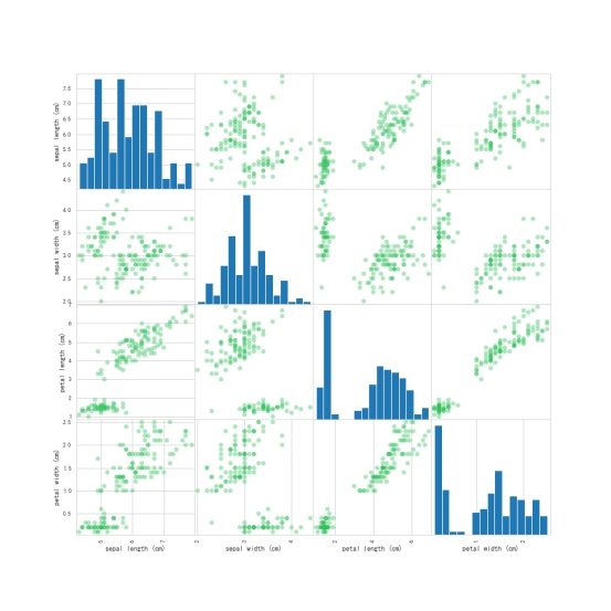

生成各特征之间关系的矩阵图

g = sns.pairplot(data=iris_df, palette=antV, hue='label')
plt.savefig("features_mat.png")
plt.show()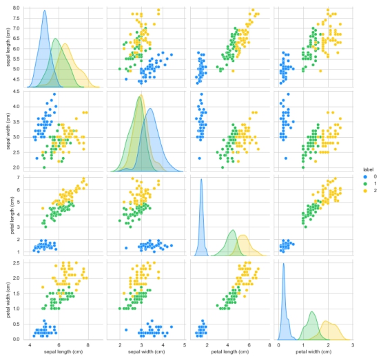

从上面绘制出的两幅图可以发现，花瓣比花萼的数据分布更有区分度，可以初步认定花瓣比花萼更适合用来作为鸢尾花分类的判断依据。

其他数据可视化

除了直方图和特征散点图矩阵外，还有其他数据可视化方法。

下面通过Violinplot 和 Pointplot，分别从数据分布和斜率，观察各特征与品种之间的关系

violinplot绘制小提琴图

f, axes = plt.subplots(2, 2, figsize=(8, 8), sharex=True)
sns.despine(left=True)
sns.violinplot(x='label', y='sepal length (cm)', data=iris_df, palette=antV, ax=axes[0, 0])
sns.violinplot(x='label', y='sepal width (cm)', data=iris_df, palette=antV, ax=axes[0, 1])
sns.violinplot(x='label', y='petal length (cm)', data=iris_df, palette=antV, ax=axes[1, 0])
sns.violinplot(x='label', y='petal width (cm)', data=iris_df, palette=antV, ax=axes[1, 1])
plt.savefig("violin.png")
plt.show()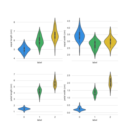

pointplot绘制


f, axes = plt.subplots(2, 2, figsize=(12, 8), sharex=True)
sns.despine(left=True)

sns.pointplot(x='label', y='sepal length (cm)', data=iris_df,  color=antV[0], ax=axes[0, 0])
sns.pointplot(x='label', y='sepal width (cm)', data=iris_df, color=antV[0], ax=axes[0, 1])
sns.pointplot(x='label', y='petal length (cm)', data=iris_df, color=antV[0], ax=axes[1, 0])
sns.pointplot(x='label', y='petal width (cm)', data=iris_df, color=antV[0], ax=axes[1, 1])
plt.savefig("pointplot.png")
plt.show()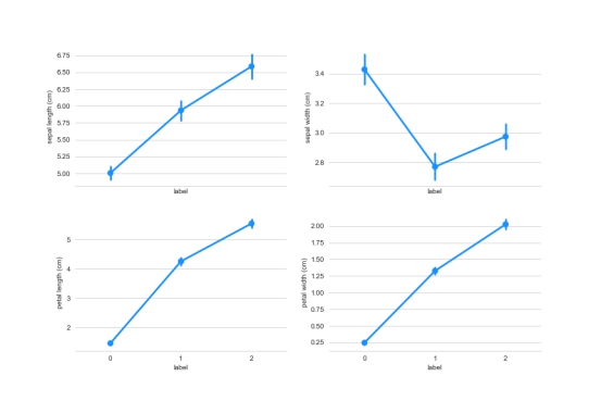

线性回归可视化

分别基于花萼和花瓣做线性回归的可视化：

g = sns.lmplot(data=iris_df, x='sepal width (cm)', y='sepal length (cm)', palette=antV, hue='label')
plt.savefig("lm_sepal.png")
plt.show()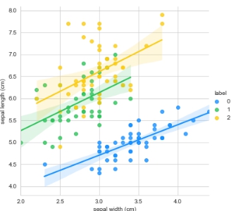

g = sns.lmplot(data=iris_df, x='petal width (cm)', y='petal length (cm)', palette=antV, hue='label')
plt.savefig("lm_petal.png")
plt.show()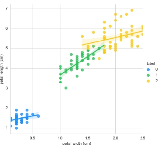

热力矩阵图

通过热图可以找出数据集中不同特征之间的相关性，高正值或负值表明特征具有高度相关性。

fig=plt.gcf()
fig.set_size_inches(12, 8)
fig=sns.heatmap(iris_df.corr(), annot=True, cmap='GnBu', linewidths=1, linecolor='k', square=True, mask=False, vmin=-1, vmax=1, cbar_kws={"orientation": "vertical"}, cbar=True)
plt.savefig("freatures_hm.png")
plt.show()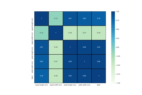

从热图也可以明显看出，花萼的宽度和长度不相关，而花瓣的宽度和长度则高度相关。

聚类可视化

from collections import Counter, defaultdict
import matplotlib
import matplotlib.pyplot as plt
import numpy as np 
matplotlib.rcParams['font.sans-serif'] = ['SimHei']

style_list = ['o', '^', '*']       # 设置点的不同形状，不同形状默认颜色不同，也可自定义
data = iris_dataset.data
labels = iris_dataset.target_names
cc = defaultdict(list)

for i, d in enumerate(data):
    cc[labels[int(i/50)]].append(d) 
p_list = []
c_list = []
 
for each in [0, 2]:
    for i, (c, ds) in enumerate(cc.items()):
        draw_data = np.array(ds)
        p = plt.plot(draw_data[:, each], draw_data[:, each+1], style_list[i])
        p_list.append(p)
        c_list.append(c)
 
    plt.legend(map(lambda x: x[0], p_list), c_list)
    plt.title('鸢尾花花瓣的长度和宽度') if each else plt.title('鸢尾花花萼的长度和宽度')
    plt.xlabel('花瓣的长度(cm)') if each else plt.xlabel('花萼的长度(cm)')
    plt.ylabel('花瓣的宽度(cm)') if each else plt.ylabel('花萼的宽度(cm)')
    plt.show()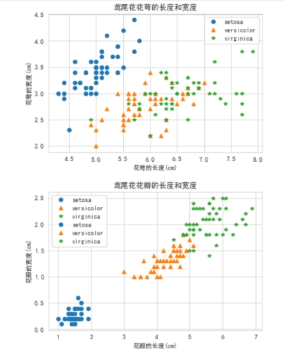

from sklearn.cluster import KMeans
import pandas as pd
kms = KMeans(n_clusters=3)
kms.fit(iris_dataset.data,iris_dataset.target)
predicted = kms.predict(iris_dataset.data)

names = ['花萼-length', '花萼-width', '花瓣-length', '花瓣-width'] 
df = pd.DataFrame(iris_dataset.data,columns=names)    
L1 = df['花瓣-length'].values   
L2 = df['花瓣-width'].values    
 
plt.scatter(L1, L2, c=predicted, marker='o',s=100,cmap=plt.cm.Paired)    
plt.title("花瓣KMeans聚类分析")    
plt.show()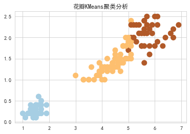

2954d7a025f3600b551a172a1856d9c

从聚类的结果也可以发现花瓣的长度和宽度区分度确实比花萼高。

03 / 决策树

此部分包含下列步骤：

划分数据集为训练集和测试集
训练决策树模型并测试
模型可视化
模型调参调优效果对比

导入相关工具包

from sklearn import tree
from sklearn import metrics
from sklearn.tree import DecisionTreeClassifier
from sklearn.model_selection import train_test_split

划分数据集为训练集和测试集

划分数据集为75%训练集25%测试集

X_train, X_test, Y_train, Y_test = train_test_split(iris_df[iris_dataset.feature_names[:]], iris_df['label'], random_state=0)

训练决策树模型并测试

从sklearn库里导入决策树分类器，设置一些参数将模型实例化，然后用训练集进行决策树模型训练，最大深度设置为3。

dt_clf = DecisionTreeClassifier(max_depth = 3, random_state = 0)
dt_clf.fit(X_train, Y_train)

> DecisionTreeClassifier(max_depth=3, random_state=0)

用测试集来预测测试准确度accuracy

````python
pred = dt_clf.predict(X_test)
print('决策树的 accuracy 为 {0}'.format(metrics.accuracy_score(pred,Y_test)))

决策树的 accuracy 为 0.9736842105263158

模型可视化

用Sklearn自带的tree包进行决策树可视化

tree.plot_tree(dt_clf);
import matplotlib.pyplot as plt
fn=iris_dataset.feature_names  # fn=['sepal length (cm)','sepal width (cm)','petal length (cm)','petal width (cm)'
cn=iris_dataset.target_names  # cn=['setosa', 'versicolor', 'virginica']
fig, axes = plt.subplots(nrows=1,ncols=1,figsize = (6,6), dpi=300)
tree.plot_tree(dt_clf,
               feature_names=fn, 
               class_names=cn,
               filled = True);
fig.savefig('vis_dt.png')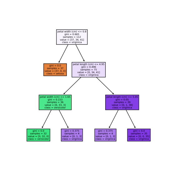

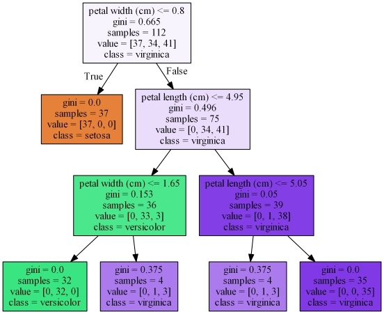
使用graphviz可视化决策树

tree.export_graphviz(dt_clf,
                     out_file="dt.dot",
                     feature_names = fn, 
                     class_names=cn,
                     filled = True)

! dot -Tpng -Gdpi=300 dt.dot -o dt_graphviz.png

![img](https://i.loli.net/2021/05/08/JHwuO5xtPbZBcEG.jpg)



#### 使用dtreeviz包进行可视化

````python
from dtreeviz.trees import dtreeviz
viz = dtreeviz(dt_clf,
               iris_dataset.data,
               iris_dataset.target,
               target_name='Species',
               feature_names=iris_dataset.feature_names,
               class_names={0:'setosa',1:'versicolor',2:'virginica'})
viz.save("dtreeviz.svg")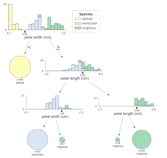

从最后这张dtreeviz生成的图可以看出，决策树通过petal width分出setosa，与versicolor和virginica分离开，再从versicolor和virginica里通过petal length和petal width分类，petal width小于1.65cm的就是versicolor，petal length大于等于5.05cm的就是virginica。

模型调参调优效果对比

经过前面数据探索已经初步确定花瓣对鸢尾花分类更有效果，下面还可以继续分析花瓣的长度和宽度对分类的影响，为了对比明显，加上了花萼的数据。

单个特征对分类准确率得分的比较

def acc_test(fn):
    acc_list=[]
    X_train, X_test, Y_train, Y_test = train_test_split(iris_df[[fn]], iris_df['label'], random_state=0)
    for i in range(1,6):
        dt_clf = DecisionTreeClassifier(max_depth = i, random_state = 0)
        dt_clf.fit(X_train, Y_train)
        pred = dt_clf.predict(X_test)
        res = metrics.accuracy_score(pred,Y_test)
        acc_list.append(res)
    return acc_list
        
acc_pl = acc_test('petal length (cm)')
acc_pw = acc_test('petal width (cm)')
acc_sl = acc_test('sepal length (cm)')
acc_sw = acc_test('sepal width (cm)')

import matplotlib
import matplotlib.pyplot as plt
matplotlib.rcParams['font.sans-serif'] = ['SimHei']

x=range(1,6)
plt.figure(figsize=(10,5))
plt.title("花萼长度vs花萼宽度vs花瓣长度vs花瓣宽度")
plt.xlabel("max_depth")
plt.xticks(rotation=45)
plt.ylabel("accuracy")
plt.plot(x,acc_pl,'-',label="花瓣长度")
plt.plot(x,acc_pw,'-',color='r',label="花瓣宽度")
plt.plot(x,acc_sl,'-',color='g',label="花萼长度")
plt.plot(x,acc_sw,'-',color='limegreen',label="花萼宽度")
plt.legend()
plt.grid()
plt.savefig("pl_pw_sl_sw.png")
plt.show()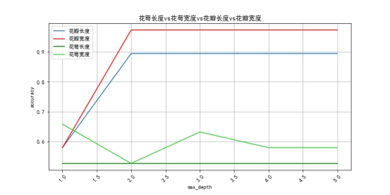

通过对比可以发现花瓣宽度比长度对分类更有效，且在最大深度为2时就收敛。

多个特征时不同最大深度对分类准确率得分的影响

acc = []
X_train, X_test, Y_train, Y_test = train_test_split(iris_df[['petal length (cm)','petal width (cm)']], iris_df['label'], random_state=0)
for i in range(1,10):
    dt_clf = DecisionTreeClassifier(max_depth = i, random_state = 0)
    dt_clf.fit(X_train, Y_train)
    pred = dt_clf.predict(X_test)
    res = metrics.accuracy_score(pred,Y_test)
    acc.append(res)
    
print(acc)
import matplotlib
import matplotlib.pyplot as plt
matplotlib.rcParams['font.sans-serif'] = ['SimHei']
y1=acc
x1=range(1,10)
plt.plot(x1,y1,label='',linewidth=2,color='limegreen',marker='o',markerfacecolor='c',markersize=8,alpha=0.9)
plt.xlabel('max_depth')
plt.ylabel('accuracy')
plt.title('花瓣宽度+花瓣长度')
plt.savefig("petal_width_lenth.png")
plt.show()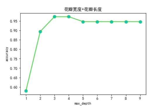

通过实验，当使用花瓣的两个特征训练决策树时，最大深度参数设置为3时较好。

04 / 随机森林

随机森林就是很多棵决策树的集成模型，由很多决策树构成的，不同决策树之间没有关联。

当我们进行分类任务时，新的输入样本进入，就让森林中的每一棵决策树分别进行判断和分类，每个决策树会得到一个自己的分类结果，决策树的分类结果中哪一个分类最多，那么随机森林就会把这个结果当做最终的结果。

随机森林模型训练

from sklearn.ensemble import RandomForestClassifier

df = pd.DataFrame(iris_dataset.data, columns=iris_dataset.feature_names)
df['target'] = iris_dataset.target
# 将数据转换为特征矩阵和目标向量
X = df.loc[:, df.columns != 'target']
y = df.loc[:, 'target'].values
# 将数据集分割为训练集和测试集
X_train, X_test, Y_train, Y_test = train_test_split(X, y, random_state=0)
# scikit-learn里的随机森林模型 (N = 100)
rf = RandomForestClassifier(n_estimators=100,
                            random_state=0)
rf.fit(X_train, Y_train)

随机森林部分可视化

这里设置了100棵树，可视化模型中的第一棵树。

fn=iris_dataset.feature_names
cn=iris_dataset.target_names
fig, axes = plt.subplots(nrows = 1,ncols = 1,figsize = (4,4), dpi=300)
tree.plot_tree(rf.estimators_[0],
               feature_names = fn, 
               class_names=cn,
               filled = True);
fig.savefig('rf_individualtree.png')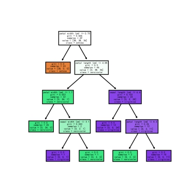

可视化其中的前五棵树

fig, axes = plt.subplots(nrows = 1,ncols = 5,figsize = (10,2), dpi=800)
for index in range(0, 5):
    tree.plot_tree(rf.estimators_[index],
                   feature_names = fn, 
                   class_names=cn,
                   filled = True,
                   ax = axes[index]);
    axes[index].set_title('Estimator: ' + str(index), fontsize = 11)
fig.savefig('rf_5trees.png')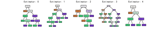

由于图太大就放不下，这里设置的小一点。

随机森林调参

下面设置从1到10棵树参数进行随机森林的训练，对比不同参数下的准确率：

acc_rf = []
for i in range(1,10):
    rf = RandomForestClassifier(n_estimators=i,
                                random_state=0)
    rf.fit(X_train, Y_train)
    pred = rf.predict(X_test)
    acc_rf.append(metrics.accuracy_score(pred,Y_test))

import matplotlib
import matplotlib.pyplot as plt
matplotlib.rcParams['font.sans-serif'] = ['SimHei']

x=range(1,10)
plt.figure(figsize=(10,5))
plt.title("随机森林")
plt.xlabel("n_estimators")
plt.xticks(rotation=45)
plt.ylabel("accuracy")
plt.plot(x,acc_rf,'-',color='limegreen',marker='o',markerfacecolor='c',markersize=6)
plt.grid()
plt.savefig("rf_acc_curve.png")
plt.show()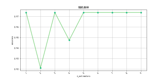

可以发现当随机森林参数设置为5之后分类准确率就基本稳定了，且其最高准确率和决策树一样，都是97.37%。

一点感想

决策树这类传统机器学习算法有极高的可解释性，可能有助于应用在深度学习的可解释性上，或许可以在帮助人们理解深度学习如何决策的方面作为辅助模型进行使用。

ML/DL 数据挖掘

Python 数据挖掘决策树随机森林鸢尾花分类

本博客所有文章除特别声明外，均采用 CC BY-SA 4.0 协议，转载请注明出处！

北大法宝法律文书数据爬取方案上一篇

编译原理2-词法分析下一篇

	sepal length (cm)	sepal width (cm)	petal length (cm)	petal width (cm)	label
0	5.1	3.5	1.4	0.2	0
1	4.9	3.0	1.4	0.2	0
2	4.7	3.2	1.3	0.2	0
3	4.6	3.1	1.5	0.2	0
4	5.0	3.6	1.4	0.2	0
…	…	…	…	…	…
145	6.7	3.0	5.2	2.3	2
146	6.3	2.5	5.0	1.9	2
147	6.5	3.0	5.2	2.0	2
148	6.2	3.4	5.4	2.3	2
149	5.9	3.0	5.1	1.8	2

	sepal length (cm)	sepal width (cm)	petal length (cm)	petal width (cm)	label
0	5.1	3.5	1.4	0.2	0
1	4.9	3.0	1.4	0.2	0
2	4.7	3.2	1.3	0.2	0
3	4.6	3.1	1.5	0.2	0
4	5.0	3.6	1.4	0.2	0
…	…	…	…	…	…
145	6.7	3.0	5.2	2.3	2
146	6.3	2.5	5.0	1.9	2
147	6.5	3.0	5.2	2.0	2
148	6.2	3.4	5.4	2.3	2
149	5.9	3.0	5.1	1.8	2

	sepal length (cm)	sepal width (cm)	petal length (cm)	petal width (cm)	label
0	5.1	3.5	1.4	0.2	0
1	4.9	3.0	1.4	0.2	0
2	4.7	3.2	1.3	0.2	0
3	4.6	3.1	1.5	0.2	0
4	5.0	3.6	1.4	0.2	0
…	…	…	…	…	…
145	6.7	3.0	5.2	2.3	2
146	6.3	2.5	5.0	1.9	2
147	6.5	3.0	5.2	2.0	2
148	6.2	3.4	5.4	2.3	2
149	5.9	3.0	5.1	1.8	2